Abstract
RNA-seq analysis involves multiple steps from processing raw sequencing data to identifying, organizing, annotating, and reporting differentially expressed genes. bcbio is an open source, community-maintained framework providing automated and scalable RNA-seq methods for identifying gene abundance counts. We have developed bcbioRNASeq, a Bioconductor package that provides ready-to-render templates and wrapper functions to post-process bcbio output data. bcbioRNASeq automates the generation of high-level RNA-seq reports, including identification of differentially expressed genes, functional enrichment analysis and quality control analysis.
Introduction
For a high-level overview of our bcbio RNA-seq
analysis pipeline, including detailed explanation of the
bcbioRNASeq S4 class definition, first consult our workflow
paper published in F1000 Research (Steinbaugh et al. 2018). This vignette is
focused on more advanced usage and edge cases that a user may encounter
when attempting to load a bcbio dataset and perform downstream quality
control analysis.
Note: if you use bcbioRNASeq in published research, please include this citation:
citation("bcbioRNASeq")## To cite bcbioRNASeq in publications use:
##
## Steinbaugh MJ, Pantano L, Kirchner RD, Barrera V, Chapman BA, Piper
## ME, Mistry M, Khetani RS, Rutherford KD, Hoffman O, Hutchinson JN, Ho
## Sui SJ. (2018). bcbioRNASeq: R package for bcbio RNA-seq analysis.
## F1000Research, 6:1976. URL
## https://f1000research.com/articles/6-1976/v2. DOI
## 10.12688/f1000research.12093.2.
##
## A BibTeX entry for LaTeX users is
##
## @Article{,
## title = {{bcbioRNASeq}: {R} package for bcbio {RNA-seq} analysis},
## author = {Michael J. Steinbaugh and Lorena Pantano and Rory D. Kirchner and Victor Barrera and Brad A. Chapman and Mary E. Piper and Meeta Mistry and Radhika S. Khetani and Kayleigh D. Rutherford and Oliver Hofmann and John N. Hutchinson and Shannan J. Ho Sui},
## journal = {F1000Research},
## volume = {6},
## number = {1976},
## year = {2018},
## url = {https://f1000research.com/articles/6-1976/v2},
## doi = {10.12688/f1000research.12093.2},
## }
## nolint start
suppressPackageStartupMessages({
    library(basejump)
    library(bcbioRNASeq)
})
## nolint end
Loading bcbio data
The bcbioRNASeq constructor function is the main
interface connecting bcbio] output data to interactive use in R. It is highly customizable and
supports a number of options for advanced use cases. Consult the
documentation for additional details.
help(topic = "bcbioRNASeq", package = "bcbioRNASeq")Upload directory
We have designed the constructor to work as simply as possible by
default. The only required argument is uploadDir, the path
to the bcbio final upload directory specified with upload:
in the YAML configuration. Refer to the bcbio
configuration documentation for detailed information on how to set
up a bcbio run, which is outside the scope of this vignette.
For example, let’s load up the example bcbio dataset stored internally in the package.
uploadDir <- system.file("extdata", "bcbio", package = "bcbioRNASeq")bcbio outputs RNA-seq data in a standardized directory structure, which is described in detail in our workflow paper.
sort(list.files(path = uploadDir, full.names = FALSE, recursive = TRUE))## [1] "2018-03-18_GSE65267-merged/bcbio-nextgen-commands.log"
## [2] "2018-03-18_GSE65267-merged/bcbio-nextgen.log"
## [3] "2018-03-18_GSE65267-merged/combined.counts"
## [4] "2018-03-18_GSE65267-merged/programs.txt"
## [5] "2018-03-18_GSE65267-merged/project-summary.yaml"
## [6] "2018-03-18_GSE65267-merged/tx2gene.csv"
## [7] "control_rep1/salmon/quant.sf"
## [8] "control_rep2/salmon/quant.sf"
## [9] "control_rep3/salmon/quant.sf"
## [10] "fa_day7_rep1/salmon/quant.sf"
## [11] "fa_day7_rep2/salmon/quant.sf"
## [12] "fa_day7_rep3/salmon/quant.sf"
## [13] "sample_metadata.csv"Counts level
By default, bcbioRNASeq
imports counts at gene level, which are required for standard
differential expression analysis (level = "genes"). For
pseudo-aligned counts (e.g. Salmon, Kallisto, Sailfish)
(Bray et al. 2016; Patro, Mount, and Kingsford
2014; Patro et al. 2017), tximport (Soneson, Love, and Robinson 2016) is used
internally to aggregate transcript-level counts to gene-level counts,
and generates length-scaled transcripts per million (TPM) values. For
aligned counts processed with featureCounts
(Liao, Smyth, and Shi 2014) (e.g. STAR, HISAT2) (Dobin et al. 2013; Dobin and Gingeras 2016; Kim,
Langmead, and Salzberg 2015), these values are already returned
at gene level, and therefore not handled by tximport. Once
the gene-level counts are imported during the bcbioRNASeq
call, the DESeq2
package (Love, Huber, and Anders 2014) is
then used to generate an internal DESeqDataSet from which
we derive normalized and variance-stabilized counts.
object <- bcbioRNASeq(uploadDir = uploadDir, level = "genes")
print(object)
## bcbioRNASeq 0.6.2 with 100 rows and 6 columns
## uploadDir: /private/var/folders/l1/8y8sjzmn15v49jgrqglghcfr0000gn/T/Rtmp7t0ccV/temp_libpathb0f511e0f2fd/bcbioRNASeq/extdata/bcbio
## dates(2): 2018-03-18 2024-03-28
## level: genes
## caller: salmon
## organism: Mus musculus
## interestingGroups: sampleName
## class: RangedSummarizedExperiment
## dim: 100 6
## metadata(27): allSamples bcbioCommandsLog ... wd yaml
## assays(6): counts aligned ... normalized vst
## rownames(100): ENSMUSG00000000001 ENSMUSG00000000003 ...
## ENSMUSG00000062661 ENSMUSG00000074340
## rowData names(0):
## colnames(6): control_rep1 control_rep2 ... fa_day7_rep2 fa_day7_rep3
## colData names(26): averageInsertSize averageReadLength ... treatment
## x5x3BiasAlternatively, if you want to perform transcript-aware analysis, such
as differential exon usage or splicing analysis, transcript-level counts
can be obtained using level = "transcripts". Note that when
counts are loaded at transcript level, TPMs are generated with tximport
internally, but no additional normalizations or transformations normally
calculated for gene-level counts with DESeq2 are generated.
object <- bcbioRNASeq(uploadDir = uploadDir, level = "transcripts", fast = TRUE)
print(object)
## bcbioRNASeq 0.6.2 with 100 rows and 6 columns
## uploadDir: /private/var/folders/l1/8y8sjzmn15v49jgrqglghcfr0000gn/T/Rtmp7t0ccV/temp_libpathb0f511e0f2fd/bcbioRNASeq/extdata/bcbio
## dates(2): 2018-03-18 2024-03-28
## level: transcripts
## caller: salmon
## organism: Mus musculus
## interestingGroups: sampleName
## fast: TRUE
## class: RangedSummarizedExperiment
## dim: 100 6
## metadata(26): allSamples bcbioCommandsLog ... wd yaml
## assays(3): counts avgTxLength tpm
## rownames(100): ENSMUST00000000001 ENSMUST00000000003 ...
## ENSMUST00000000674 ENSMUST00000000687
## rowData names(0):
## colnames(6): control_rep1 control_rep2 ... fa_day7_rep2 fa_day7_rep3
## colData names(26): averageInsertSize averageReadLength ... treatment
## x5x3BiasExpression callers
Since bcbio is flexible and supports a number of expression callers,
we have provided advanced options in the bcbioRNASeq
constructor to support a variety of workflows using the
caller argument. Salmon, Kallisto, and Sailfish counts are
supported at either gene or transcript level. Internally, these are
loaded using tximport. STAR and HISAT2 aligned counts processed with
featureCounts are also supported, but only at gene level.
object <- bcbioRNASeq(uploadDir = uploadDir, caller = "star", fast = TRUE)
print(object)
## bcbioRNASeq 0.6.2 with 100 rows and 6 columns
## uploadDir: /private/var/folders/l1/8y8sjzmn15v49jgrqglghcfr0000gn/T/Rtmp7t0ccV/temp_libpathb0f511e0f2fd/bcbioRNASeq/extdata/bcbio
## dates(2): 2018-03-18 2024-03-28
## level: genes
## caller: star
## organism: Mus musculus
## interestingGroups: sampleName
## fast: TRUE
## class: RangedSummarizedExperiment
## dim: 100 6
## metadata(25): allSamples bcbioCommandsLog ... wd yaml
## assays(1): counts
## rownames(100): ENSMUSG00000000001 ENSMUSG00000000003 ...
## ENSMUSG00000000563 ENSMUSG00000000567
## rowData names(0):
## colnames(6): control_rep1 control_rep2 ... fa_day7_rep2 fa_day7_rep3
## colData names(26): averageInsertSize averageReadLength ... treatment
## x5x3BiasSample selection and metadata
If you’d like to load up only a subset of samples, this can be done
easily using the samples argument. Note that the
character vector declared here must match the
description column specified in the sample metadata.
Conversely, if you’re working with a large dataset and you simply want
to drop a few samples, this can be accomplished with the
censorSamples argument.
When working with a bcbio run that has incorrect or outdated
metadata, the simplest way to fix this issue is to pass in new metadata
from an external spreadsheet (CSV or Excel) using the
sampleMetadataFile argument. Note that this can also be
used to subset the bcbio dataset, similar to the samples
argument (see above), based on the rows that are included in the
spreadsheet.
sampleMetadataFile <- file.path(uploadDir, "sample_metadata.csv")
stopifnot(file.exists(sampleMetadataFile))
import(sampleMetadataFile)
## fileName description treatment day
## 1 control_rep1_R1.fastq.gz control_rep1 control 0
## 2 control_rep2_R1.fastq.gz control_rep2 control 0
## 3 control_rep3_R1.fastq.gz control_rep3 control 0
## 4 fa_day7_rep1_R1.fastq.gz fa_day7_rep1 folic acid 7
## 5 fa_day7_rep2_R1.fastq.gz fa_day7_rep2 folic acid 7
## 6 fa_day7_rep3_R1.fastq.gz fa_day7_rep3 folic acid 7
object <- bcbioRNASeq(
    uploadDir = uploadDir,
    sampleMetadataFile = sampleMetadataFile,
    fast = TRUE
)
sampleData(object)
## DataFrame with 6 rows and 5 columns
## day fileName sampleName treatment
## <factor> <factor> <factor> <factor>
## control_rep1 0 control_rep1_R1.fastq.gz control_rep1 control
## control_rep2 0 control_rep2_R1.fastq.gz control_rep2 control
## control_rep3 0 control_rep3_R1.fastq.gz control_rep3 control
## fa_day7_rep1 7 fa_day7_rep1_R1.fastq.gz fa_day7_rep1 folic acid
## fa_day7_rep2 7 fa_day7_rep2_R1.fastq.gz fa_day7_rep2 folic acid
## fa_day7_rep3 7 fa_day7_rep3_R1.fastq.gz fa_day7_rep3 folic acid
## interestingGroups
## <factor>
## control_rep1 control_rep1
## control_rep2 control_rep2
## control_rep3 control_rep3
## fa_day7_rep1 fa_day7_rep1
## fa_day7_rep2 fa_day7_rep2
## fa_day7_rep3 fa_day7_rep3Genome annotations
When analyzing a dataset against a well-annotated genome, we
recommend importing the corresponding metadata using AnnotationHub
and ensembldb. This
functionality is natively supported in the bcbioRNASeq
constructor with using the organism,
ensemblRelease, and genomeBuild arguments. For
example, with our internal bcbio dataset, we’re analyzing counts
generated against the Ensembl
Mus musculus GRCm38 genome build (release 87). These parameters
can be defined in the object load call to ensure that the annotations
match up exactly with the genome used.
object <- bcbioRNASeq(
    uploadDir = uploadDir,
    level = "genes",
    organism = "Mus musculus",
    genomeBuild = "GRCm38",
    ensemblRelease = 87L
)
This will return a GRanges object using the GenomicRanges
package (Lawrence et al. 2013), which
contains coordinates and rich metadata for each gene or transcript.
These annotations are accessible with the rowRanges and
rowData functions defined in the SummarizedExperiment
package (Huber et al. 2015).
summary(rowRanges(object))## [1] "GRanges object with 100 ranges and 8 metadata columns"
summary(rowData(object))## [1] "DataFrame object of length 8 with 0 metadata columns"Alternatively, transcript-level annotations can also be obtained automatically using this method.
When working with a dataset generated against a poorly-annotated or
non-standard genome, we provide a fallback method for loading gene
annotations from a general
feature format (GFF) file with the gffFile argument. If
possible, we recommend providing a general transfer format (GTF) file,
which is identical to GFF version 2. GFFv3 is more complicated and
non-standard, but Ensembl GFFv3 files are also supported.
If your dataset contains transgenes (e.g. EGFP, TDTOMATO), these
features can be defined with the transgeneNames argument,
which will automatically populate the rowRanges slot with
placeholder metadata.
We recommend loading up data per genome in its own
bcbioRNASeq object when possible, so that rich metadata can
be imported easily. In the edge case where you need to look at multiple
genomes simultaneously, set organism = NULL, and
bcbioRNASeq will skip the gene annotation acquisition step.
Refer to the the GenomicRanges
and SummarizedExperiment
package documentation for more details on working with the genome
annotations defined in the rowRanges slot of the object.
Here are some useful examples:
seqnames(object)## factor-Rle of length 100 with 64 runs
## Lengths: 1 1 1 1 1 1 1 1 5 1 1 ... 1 1 1 2 1 1 1 1 2 1
## Values : 3 X 16 11 6 13 4 9 11 17 5 ... 6 5 9 11 8 11 7 15 2 3
## Levels(86): 3 X 16 7 ... CHR_MG3836_PATCH CHR_MG3496_PATCH CHR_MG3172_PATCH
ranges(object)## IRanges object with 100 ranges and 0 metadata columns:
## start end width
## <integer> <integer> <integer>
## ENSMUSG00000000001 108107280 108146146 38867
## ENSMUSG00000000003 77837901 77853623 15723
## ENSMUSG00000000028 18780447 18811987 31541
## ENSMUSG00000000049 108343354 108414396 71043
## ENSMUSG00000000058 17281185 17289115 7931
## ... ... ... ...
## ENSMUSG00000048583 142650766 142666816 16051
## ENSMUSG00000055022 92051165 92341967 290803
## ENSMUSG00000061689 156613705 156764363 150659
## ENSMUSG00000062661 31245823 31295989 50167
## ENSMUSG00000074340 105973711 105987423 13713
strand(object)## factor-Rle of length 100 with 42 runs
## Lengths: 3 7 1 3 2 2 1 2 3 1 2 6 2 3 2 3 ... 2 3 1 4 1 1 2 2 2 4 2 2 1 4 2 4
## Values : - + - + - + - + - + - + - + - + ... - + - + - + - + - + - + - + - +
## Levels(3): + - *Variance stabilization
During the bcbioRNASeq constructor call, log2 variance
stabilizaton of gene-level counts can be calculated automatically, and
is recommended. This is performed internally by the DESeq2 package,
using the varianceStabilizingTransformation and/or
rlog functions. These transformations will be slotted into
assays.
##   control_rep1     control_rep2     control_rep3     fa_day7_rep1
##  Min.   : 4.919   Min.   : 4.919   Min.   : 4.919   Min.   : 4.919
##  1st Qu.: 4.919   1st Qu.: 4.919   1st Qu.: 4.919   1st Qu.: 4.919
##  Median : 6.051   Median : 5.658   Median : 6.009   Median : 6.237
##  Mean   : 6.713   Mean   : 6.706   Mean   : 6.715   Mean   : 6.762
##  3rd Qu.: 7.990   3rd Qu.: 8.239   3rd Qu.: 7.815   3rd Qu.: 8.239
##  Max.   :12.215   Max.   :12.972   Max.   :11.818   Max.   :11.764
##   fa_day7_rep2     fa_day7_rep3
##  Min.   : 4.919   Min.   : 4.919
##  1st Qu.: 5.101   1st Qu.: 4.919
##  Median : 6.216   Median : 6.185
##  Mean   : 6.754   Mean   : 6.789
##  3rd Qu.: 8.033   3rd Qu.: 7.930
##  Max.   :12.086   Max.   :11.997
Use case dataset
To demonstrate the functionality and configuration of the package, we have taken an experiment from the Gene Expression Omnibus (GEO) public repository of expression data to use as an example use case. The RNA-seq data is from a study of acute kidney injury in a mouse model (GSE65267) (Craciun et al. 2016). The study aims to identify differentially expressed genes in progressive kidney fibrosis and contains samples from mouse kidneys at several time points (n = 3, per time point) after folic acid treatment. From this dataset, we are using a subset of the samples for our use case: before folic acid treatment, and 1, 3, 7 days after treatment.
For the vignette, we are loading a pre-computed version of the
example bcbioRNASeq object used in our workflow paper.
object <- import(
    con = cacheUrl(
        pasteUrl(
            "github.com",
            "hbc",
            "bcbioRNASeq",
            "raw",
            "f1000v2",
            "data",
            "bcb.rda",
            protocol = "https"
        ),
        pkg = "bcbioRNASeq"
    )
)
object <- updateObject(object)
print(object)
## bcbioRNASeq 0.6.2 with 51652 rows and 12 columns
## uploadDir: /n/data1/cores/bcbio/bcbioRNASeq/F1000v2/GSE65267-merged/final
## dates(2): 2018-03-18 2018-06-01
## level: genes
## caller: salmon
## organism: Mus musculus
## ensemblRelease: 90
## interestingGroups: day
## class: RangedSummarizedExperiment
## dim: 51652 12
## metadata(28): level caller ... previousVersion packageVersion
## assays(6): counts tpm ... rlog vst
## rownames(51652): ENSMUSG00000000001 ENSMUSG00000000003 ...
## ENSMUSG00000114967 ENSMUSG00000114968
## rowData names(7): geneId geneName ... ncbiGeneId broadClass
## colnames(12): control_rep1 control_rep2 ... fa_day7_rep2 fa_day7_rep3
## colData names(25): sampleName day ... x5x3Bias xGcSample metadata
For reference, let’s take a look at the sample metadata. By
comparison, using colData will return all sample-level
metadata, including our quality control metrics generated by bcbio. We
recommend instead using sampleData with the
clean = TRUE argument in reports, which only returns
factor columns of interest.
sampleData(object)## DataFrame with 12 rows and 7 columns
## sampleName day replicate strain tissue treatment
## <factor> <factor> <factor> <factor> <factor> <factor>
## control_rep1 control_rep1 0 1 Balb/c kidney control
## control_rep2 control_rep2 0 2 Balb/c kidney control
## control_rep3 control_rep3 0 3 Balb/c kidney control
## fa_day1_rep1 fa_day1_rep1 1 1 Balb/c kidney folic acid
## fa_day1_rep2 fa_day1_rep2 1 2 Balb/c kidney folic acid
## ... ... ... ... ... ... ...
## fa_day3_rep2 fa_day3_rep2 3 2 Balb/c kidney folic acid
## fa_day3_rep3 fa_day3_rep3 3 3 Balb/c kidney folic acid
## fa_day7_rep1 fa_day7_rep1 7 1 Balb/c kidney folic acid
## fa_day7_rep2 fa_day7_rep2 7 2 Balb/c kidney folic acid
## fa_day7_rep3 fa_day7_rep3 7 3 Balb/c kidney folic acid
## interestingGroups
## <factor>
## control_rep1 0
## control_rep2 0
## control_rep3 0
## fa_day1_rep1 1
## fa_day1_rep2 1
## ... ...
## fa_day3_rep2 3
## fa_day3_rep3 3
## fa_day7_rep1 7
## fa_day7_rep2 7
## fa_day7_rep3 7Interesting groups
Groups of interest to be used for coloring and sample grouping in the
quality control plots can be defined in the bcbioRNASeq
object using the interestingGroups argument in the
bcbioRNASeq constructor call. Assignment method support
with the interestingGroups function is also provided, which
can modify the groups of interest after the object has been created.
The interestingGroups definition defaults to
sampleName, which is automatically generated from the bcbio
description metadata for demultiplexed bulk RNA-seq
samples. In this case, the samples will be grouped and colored
uniquely.
Interesting groups must be defined using a character
vector and refer to column names defined in the colData
slot of the object. Note that the bcbioRNASeq package uses lower camel
case formatting for column names (e.g. “sampleName”), so the interesting
groups should be defined using camel case, not snake
(e.g. “sample_name”) or dotted case (e.g. “sample.name”).
This approach was inspired by the DESeq2 package, which uses the
argument intgroup in some functions, such as
plotPca for labeling groups of interest. We took this idea
and ran with it for a number of our quality control functions, which are
described in detail below.
interestingGroups(object) <- c("treatment", "day")Quality control
Our workflow paper describes the quality control process in detail.
In addition, our Quality Control R Markdown template contains
notes detailing each metric. Here were are going into more technical
detail regarding how to customize the appearance of the plots. Note that
all quality control plotting functions inherit the
interestingGroups defined inside the
bcbioRNASeq object. You can also change this dynamially for
each function call using the interestingGroups
argument.
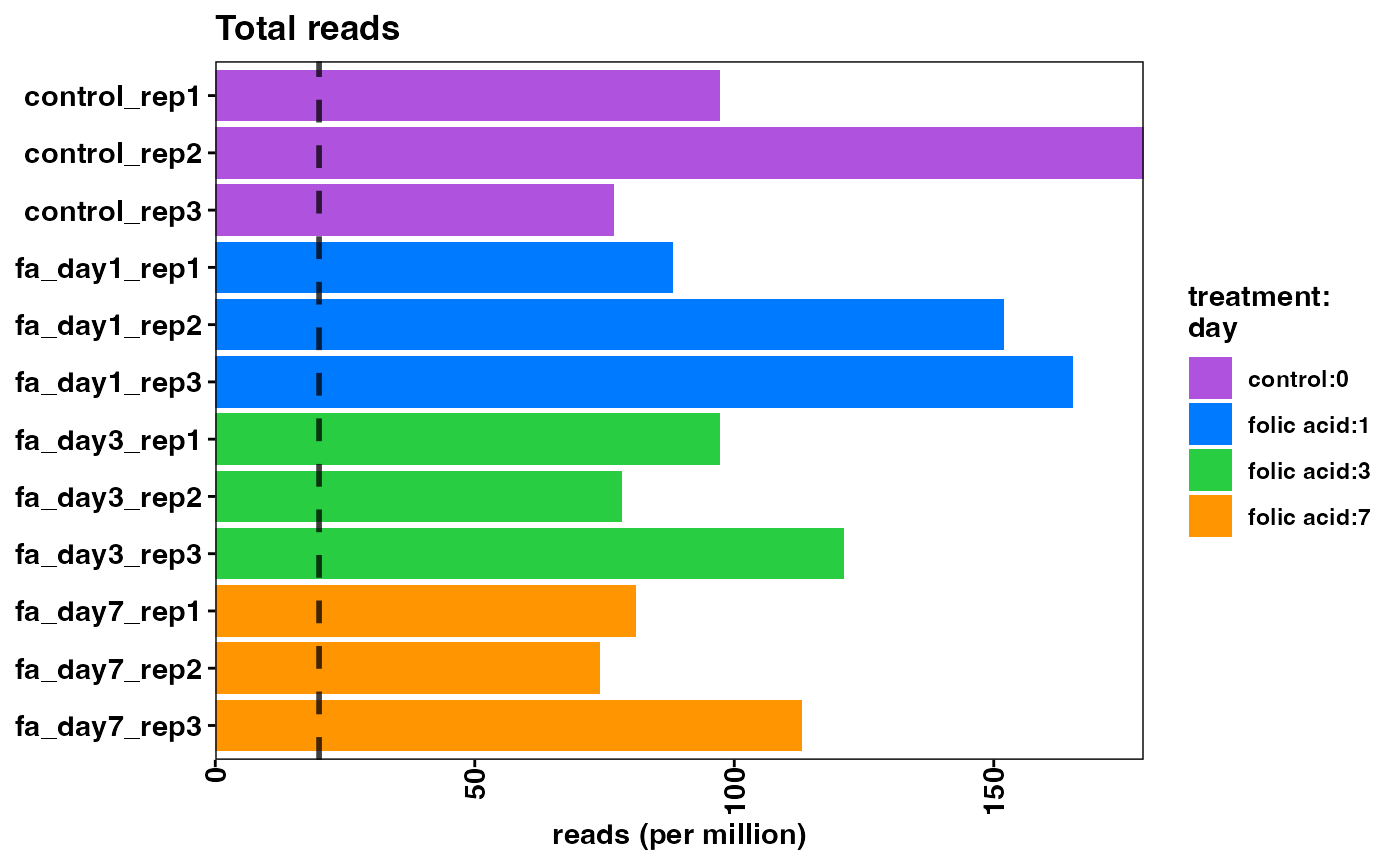
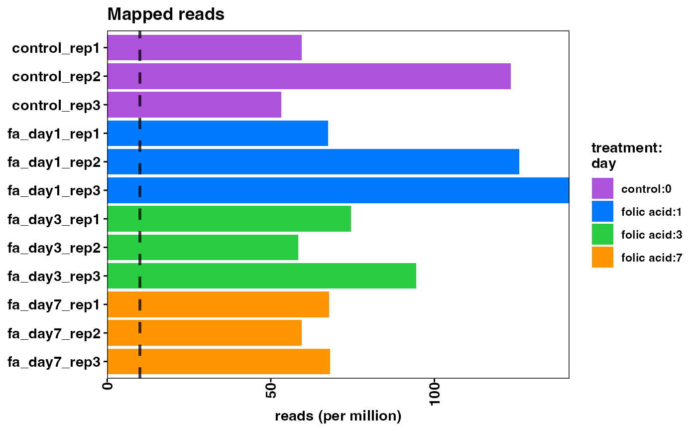
Mapping rates
Note that the overall mapping rate is relatively low per sample, while the exonic mapping rate is acceptable. High quality samples should have low intronic mapping rate, and high values are indicative of sample degradation and/or contamination.
plotMappingRate(object)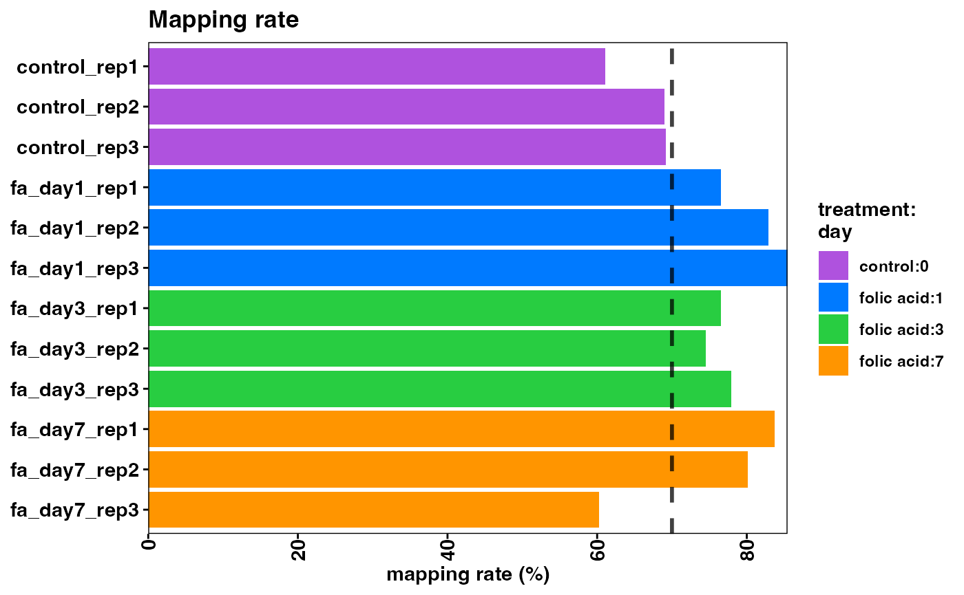
plotExonicMappingRate(object)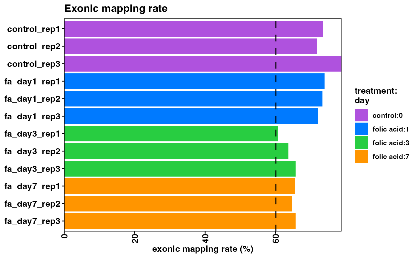
plotIntronicMappingRate(object)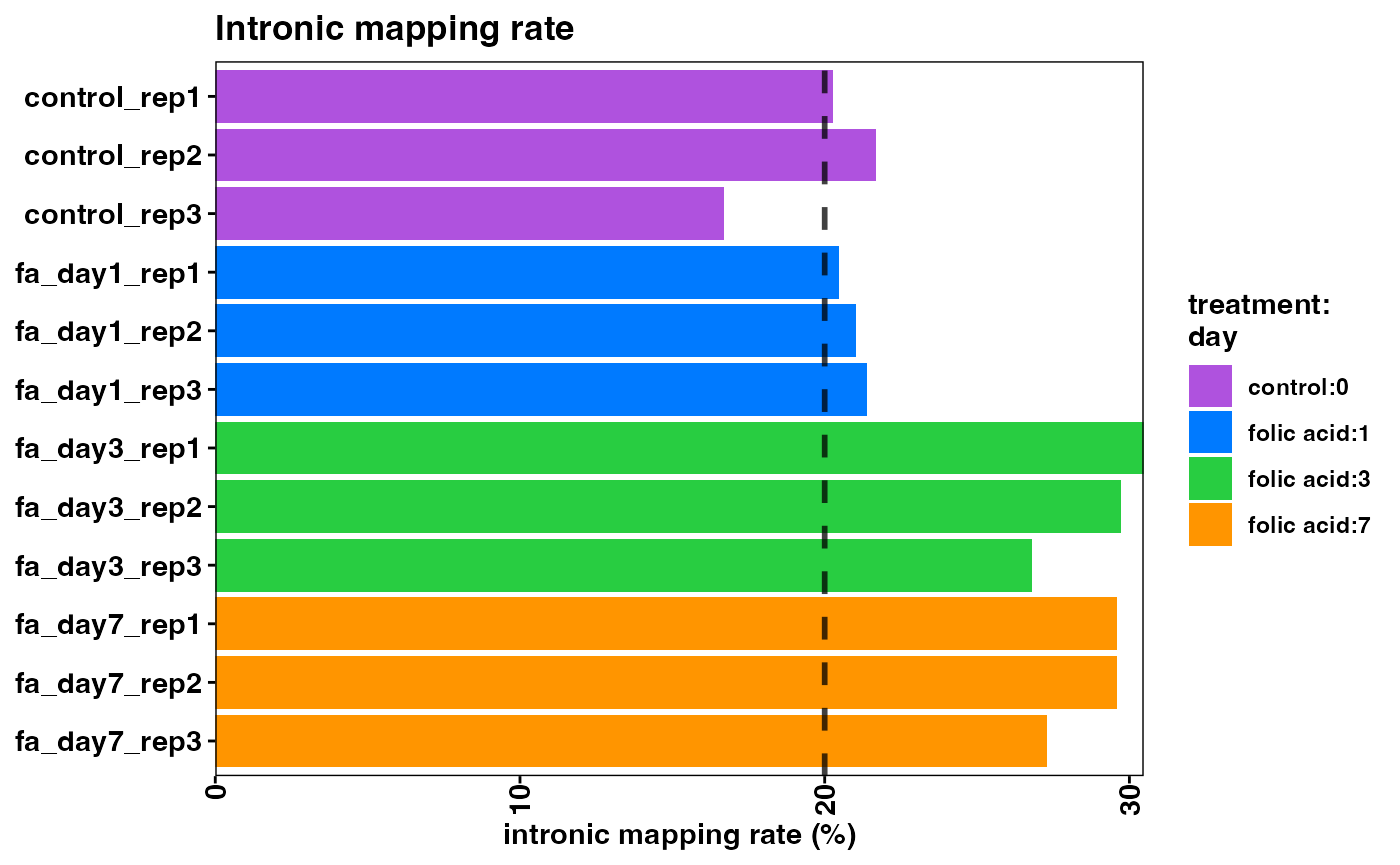
rRNA mapping rate
Note that the samples here have a high rRNA mapping rate. This can be indicative of the polyA enrichment or ribo depletion protocol not having removed all ribosomal RNA (rRNA) transcripts. This will reduce the number of biologically meaningful reads in the experiment and is best avoided.
plotRrnaMappingRate(object)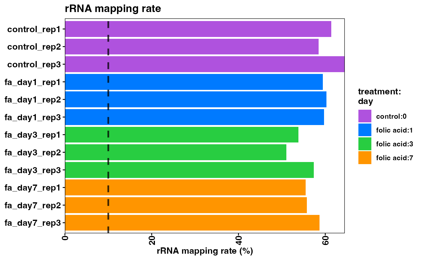
5’->3’ bias
RNA-seq data can have specific biases at either the 5’ or 3’ end of sequenced fragments. It is common to see a small amount of bias, especially if polyA enrichment was performed, or if there is any sample degradation. If a large amount of bias is observed here, be sure to analyze the samples with a Bioanalyzer and check the RIN scores.
plot5Prime3PrimeBias(object)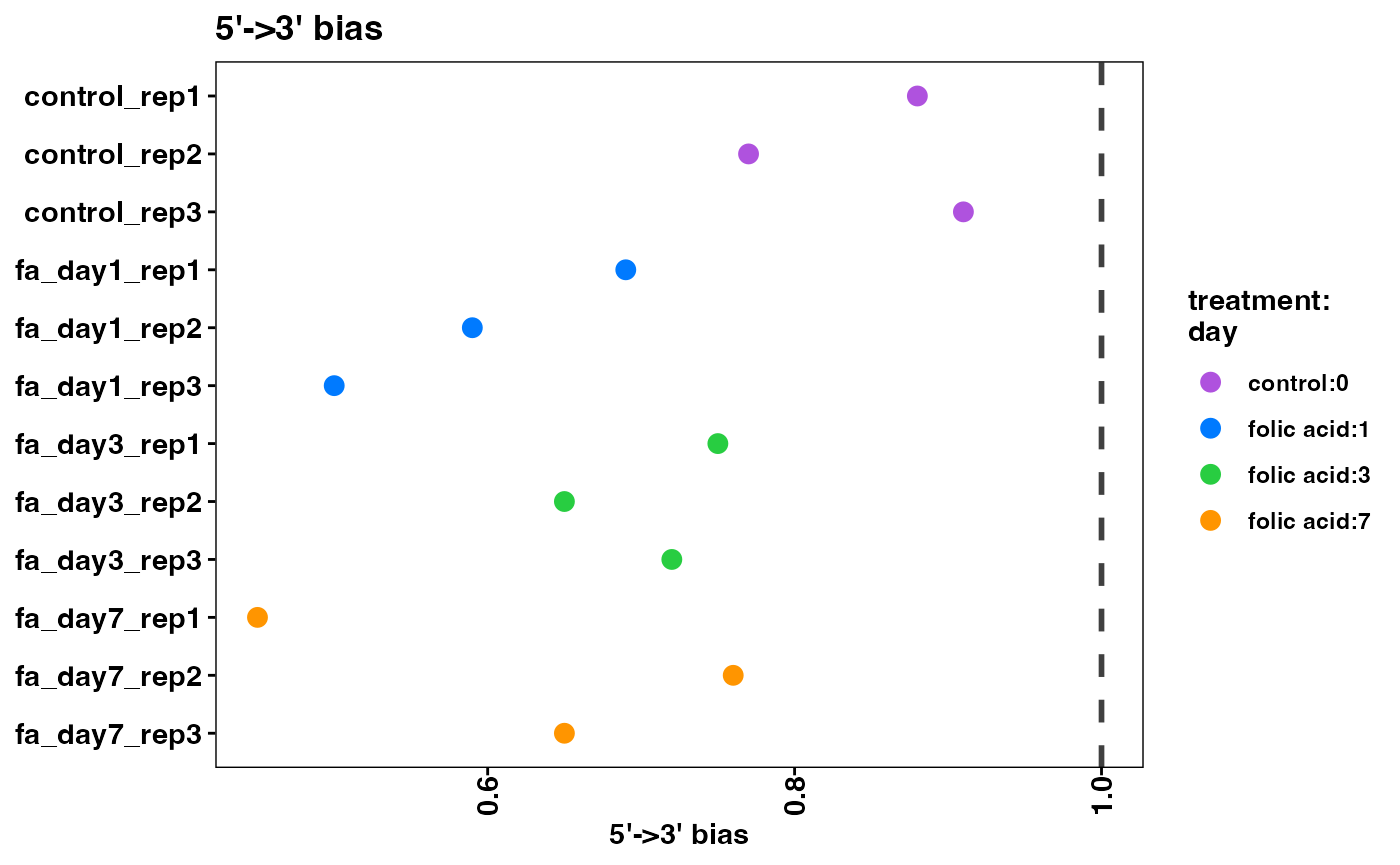
Feature (gene) distributions
plotFeaturesDetected(object)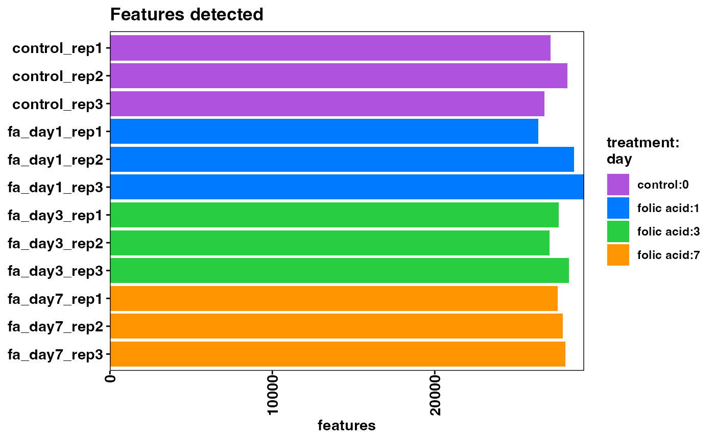
plotFeatureSaturation(object)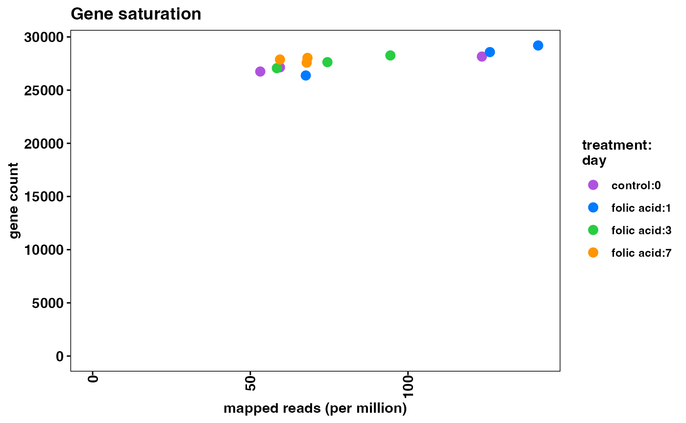
plotCountsPerFeature(object, geom = "boxplot")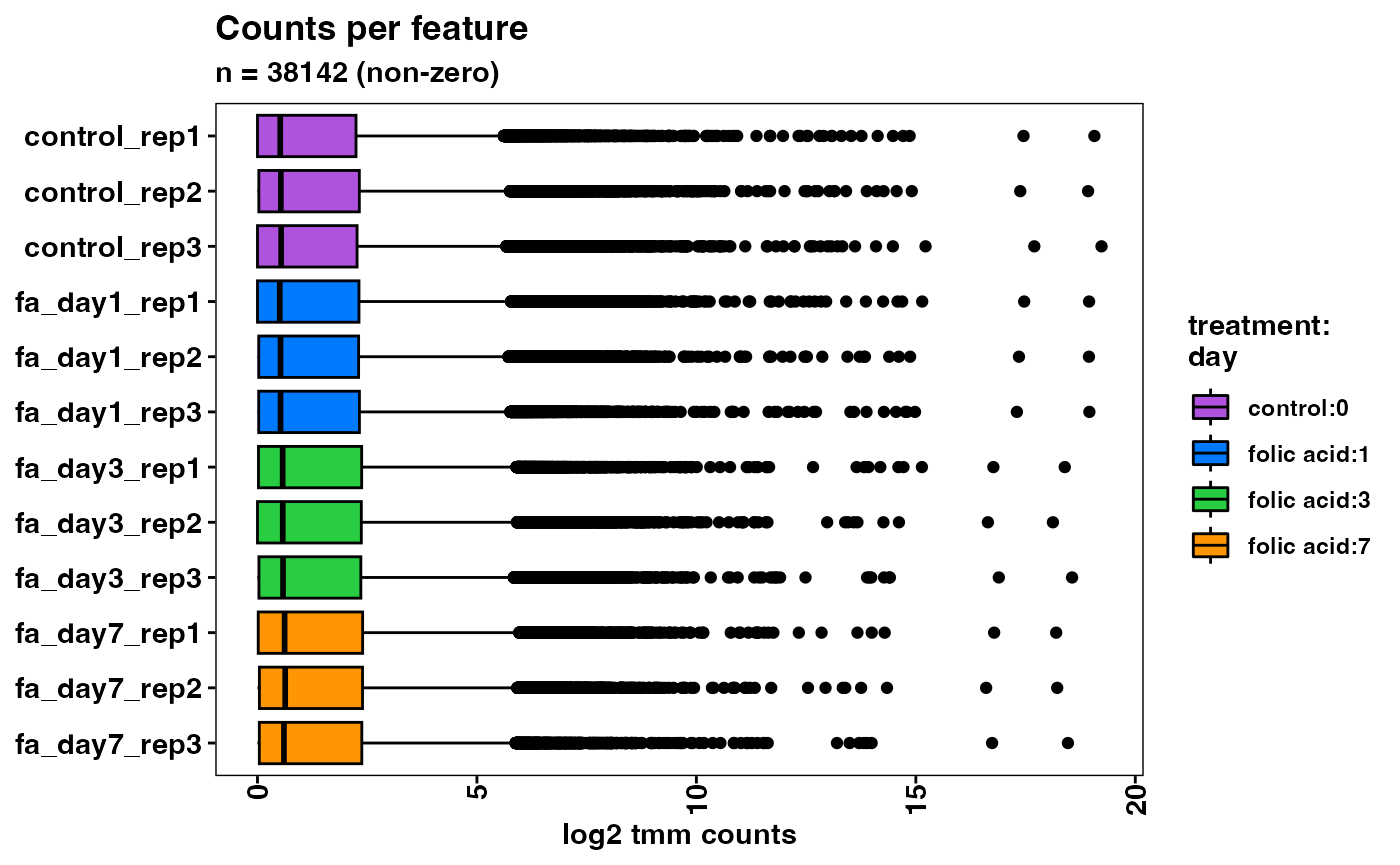
plotCountsPerFeature(object, geom = "density")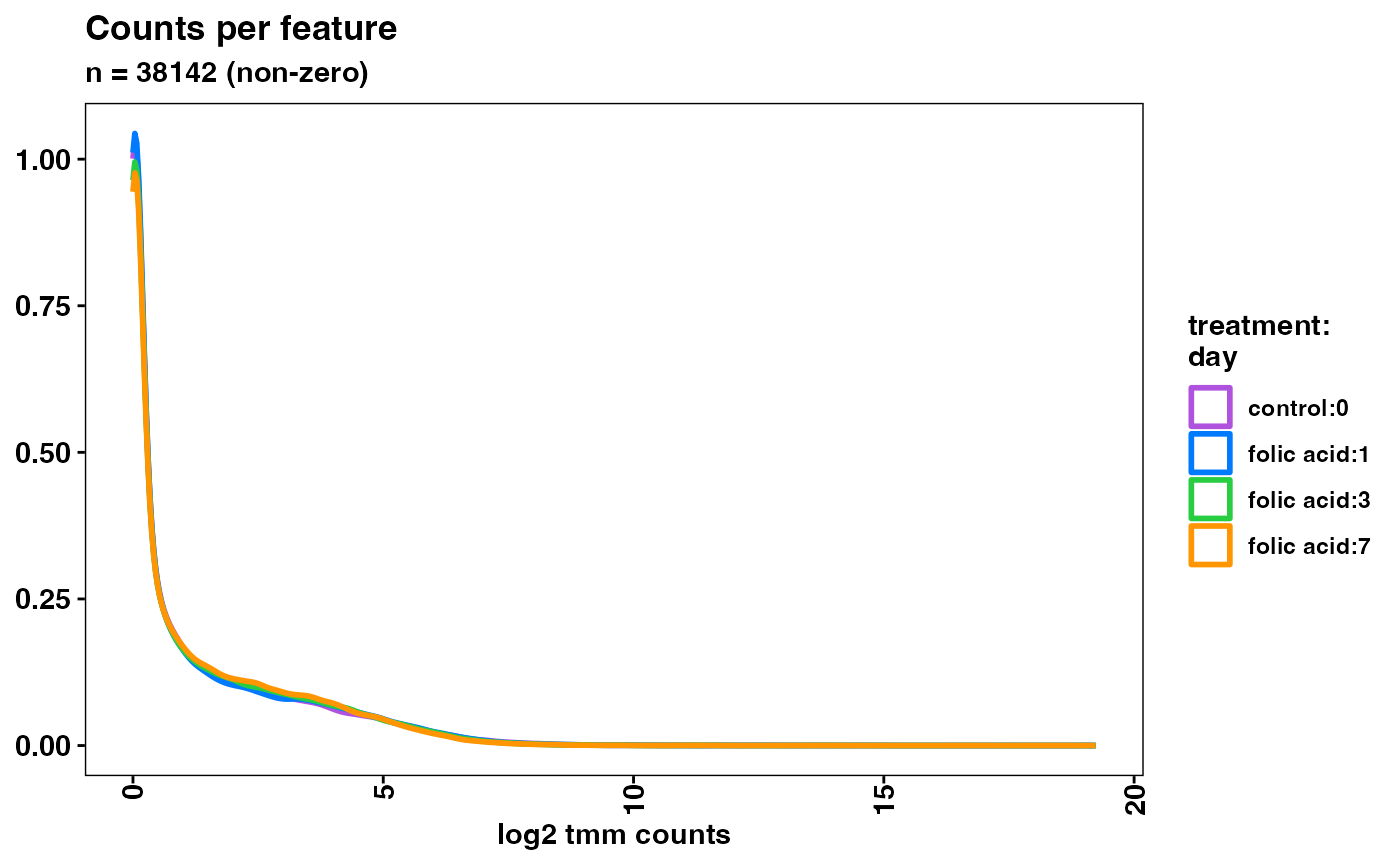
Sample similarity
We can visualize sample similarity with principal component analysis
(PCA) and hierarchical clustering of sample correlations. These
functions support multiple normalization methods with the
normalized argument.
plotPca(object)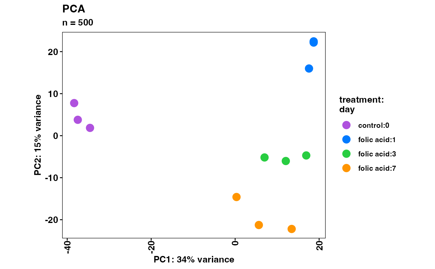
plotCorrelationHeatmap(object)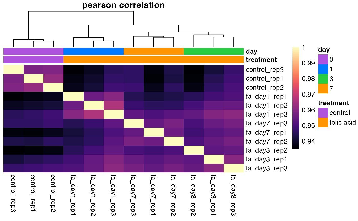
Export
The counts accessor function returns raw counts by
default. Multiple normalization methods are accessible with the
normalized argument.
rawCounts <- counts(object, normalized = FALSE)
normalizedCounts <- counts(object, normalized = TRUE)
tpm <- counts(object, normalized = "tpm")
log2VstCounts <- counts(object, normalized = "vst")
We are providing bcbioRNASeq method support for the
export function, which automatically exports matrices
defined in assays and corresponding metadata
(e.g. rowData, colData) to disk in a single
call.
## $assays
## $assays$counts
## [1] "/private/var/folders/l1/8y8sjzmn15v49jgrqglghcfr0000gn/T/Rtmp2KSeRu/assays/counts.csv"
##
## $assays$tpm
## [1] "/private/var/folders/l1/8y8sjzmn15v49jgrqglghcfr0000gn/T/Rtmp2KSeRu/assays/tpm.csv"
##
## $assays$avgTxLength
## [1] "/private/var/folders/l1/8y8sjzmn15v49jgrqglghcfr0000gn/T/Rtmp2KSeRu/assays/avgTxLength.csv"
##
## $assays$normalized
## [1] "/private/var/folders/l1/8y8sjzmn15v49jgrqglghcfr0000gn/T/Rtmp2KSeRu/assays/normalized.csv"
##
## $assays$rlog
## [1] "/private/var/folders/l1/8y8sjzmn15v49jgrqglghcfr0000gn/T/Rtmp2KSeRu/assays/rlog.csv"
##
## $assays$vst
## [1] "/private/var/folders/l1/8y8sjzmn15v49jgrqglghcfr0000gn/T/Rtmp2KSeRu/assays/vst.csv"
##
##
## $rowData
## [1] "/private/var/folders/l1/8y8sjzmn15v49jgrqglghcfr0000gn/T/Rtmp2KSeRu/rowData.csv"
##
## $colData
## [1] "/private/var/folders/l1/8y8sjzmn15v49jgrqglghcfr0000gn/T/Rtmp2KSeRu/colData.csv"
Differential expression
bcbioRNASeq integrates with DESeq2 and edgeR for differential expression.
DESeq2
To prepare our dataset for analysis, we need to coerce the
bcbioRNASeq object to a DESeqDataSet. We have
defined an S4 coercion method that uses the as function in
the package.
dds <- as(object, "DESeqDataSet")
print(dds)
## class: DESeqDataSet
## dim: 51652 12
## metadata(11): caller countsFromAbundance ... sessionInfo version
## assays(1): counts
## rownames(51652): ENSMUSG00000000001 ENSMUSG00000000003 ...
## ENSMUSG00000114967 ENSMUSG00000114968
## rowData names(7): geneId geneName ... ncbiGeneId broadClass
## colnames(12): control_rep1 control_rep2 ... fa_day7_rep2 fa_day7_rep3
## colData names(25): sampleName day ... x5x3Bias xGcSince both bcbioRNASeq and DESeqDataSet
classes extend RangedSummarizedExperiment, internally we
coerce the original bcbioRNASeq object to a
RangedSummarizedExperiment and then use the
DESeqDataSet constructor, which requires a
SummarizedExperiment with integer counts.
The source code for our bcbioRNASeq to
DESeqDataSet coercion is accessible with
getMethod.
getMethod(
    f = "coerce",
    signature = signature(from = "bcbioRNASeq", to = "DESeqDataSet")
)
We also provide a parameterized starter R Markdown template for standard DESeq2 differential expression, supporting analysis and visualization of multiple contrasts inside a single report. In our workflow paper, we also describe an example LRT analysis.
Now you can perform differential expression analysis with DESeq2. The authors of that package have provided a number of detailed, well documented references online:
edgeR
To prepare our dataset for analysis, we need to coerce the
bcbioRNASeq object to a DGEList. Similar to
our DESeq2 approach, we have defined an S4 coercion method that hands
off to edgeR.
dge <- as(object, "DGEList")
summary(dge)
## Length Class Mode
## counts 619824 -none- numeric
## samples 3 data.frame listThe source code for our bcbioRNASeq to
DGEList coercion is accessible with
getMethod.
getMethod(
    f = "coerce",
    signature = signature(from = "bcbioRNASeq", to = "DGEList")
)
Functional analysis
We provide a starter R Markdown template for gene set enrichment analysis (GSEA) and Kyoto Encyclopedia of Genes and Genomes (KEGG) pathway enrichment analysis (Kanehisa and Goto 2000; Subramanian et al. 2005), which leverages the functionality of the clusterProfiler package (Yu et al. 2012). This workflow is described in detail in our workflow paper, and is outside the scope of this advanced use vignette. For more information on functional analysis, consult the clusterProfiler vignette or Stephen Turner’s excellent DESeq2 to fgsea workflow.
R session information
utils::sessionInfo()## R version 4.3.3 (2024-02-29)
## Platform: x86_64-apple-darwin20 (64-bit)
## Running under: macOS Sonoma 14.4.1
##
## Matrix products: default
## BLAS: /Library/Frameworks/R.framework/Versions/4.3-x86_64/Resources/lib/libRblas.0.dylib
## LAPACK: /Library/Frameworks/R.framework/Versions/4.3-x86_64/Resources/lib/libRlapack.dylib; LAPACK version 3.11.0
##
## locale:
## [1] en_US.UTF-8/en_US.UTF-8/en_US.UTF-8/C/en_US.UTF-8/en_US.UTF-8
##
## time zone: America/New_York
## tzcode source: internal
##
## attached base packages:
## [1] stats4 stats graphics grDevices utils datasets methods
## [8] base
##
## other attached packages:
## [1] ensembldb_2.26.0 AnnotationFilter_1.26.0
## [3] GenomicFeatures_1.54.4 AnnotationDbi_1.64.1
## [5] bcbioRNASeq_0.6.2 syntactic_0.7.1
## [7] pipette_0.15.2 AcidSingleCell_0.4.2
## [9] AcidPlyr_0.5.4 AcidPlots_0.7.3
## [11] AcidMarkdown_0.3.0 AcidGenomes_0.8.0.9000
## [13] AcidExperiment_0.5.4 AcidBase_0.7.3
## [15] SingleCellExperiment_1.24.0 SummarizedExperiment_1.32.0
## [17] Biobase_2.62.0 GenomicRanges_1.54.1
## [19] GenomeInfoDb_1.38.8 IRanges_2.36.0
## [21] S4Vectors_0.40.2 BiocGenerics_0.48.1
## [23] MatrixGenerics_1.14.0 matrixStats_1.2.0
## [25] basejump_0.18.0 BiocStyle_2.30.0
##
## loaded via a namespace (and not attached):
## [1] RColorBrewer_1.1-3 jsonlite_1.8.8
## [3] tximport_1.30.0 magrittr_2.0.3
## [5] farver_2.1.1 rmarkdown_2.26
## [7] fs_1.6.3 BiocIO_1.12.0
## [9] zlibbioc_1.48.2 ragg_1.3.0
## [11] vctrs_0.6.5 Rsamtools_2.18.0
## [13] memoise_2.0.1 RCurl_1.98-1.14
## [15] htmltools_0.5.8 S4Arrays_1.2.1
## [17] progress_1.2.3 AnnotationHub_3.10.0
## [19] curl_5.2.1 SparseArray_1.2.4
## [21] sass_0.4.9 bslib_0.6.2
## [23] bcbioBase_0.9.0 desc_1.4.3
## [25] cachem_1.0.8 GenomicAlignments_1.38.2
## [27] mime_0.12 lifecycle_1.0.4
## [29] pkgconfig_2.0.3 Matrix_1.6-5
## [31] R6_2.5.1 fastmap_1.1.1
## [33] GenomeInfoDbData_1.2.11 shiny_1.8.1
## [35] digest_0.6.35 colorspace_2.1-0
## [37] patchwork_1.2.0 DESeq2_1.42.1
## [39] textshaping_0.3.7 RSQLite_2.3.5
## [41] labeling_0.4.3 filelock_1.0.3
## [43] fansi_1.0.6 httr_1.4.7
## [45] abind_1.4-5 compiler_4.3.3
## [47] bit64_4.0.5 withr_3.0.0
## [49] BiocParallel_1.36.0 viridis_0.6.5
## [51] DBI_1.2.2 highr_0.10
## [53] biomaRt_2.58.2 rappdirs_0.3.3
## [55] DelayedArray_0.28.0 rjson_0.2.21
## [57] tools_4.3.3 interactiveDisplayBase_1.40.0
## [59] httpuv_1.6.15 glue_1.7.0
## [61] restfulr_0.0.15 promises_1.2.1
## [63] grid_4.3.3 generics_0.1.3
## [65] gtable_0.3.4 tzdb_0.4.0
## [67] hms_1.1.3 xml2_1.3.6
## [69] utf8_1.2.4 XVector_0.42.0
## [71] BiocVersion_3.18.1 pillar_1.9.0
## [73] stringr_1.5.1 vroom_1.6.5
## [75] limma_3.58.1 later_1.3.2
## [77] dplyr_1.1.4 BiocFileCache_2.10.1
## [79] lattice_0.22-6 rtracklayer_1.62.0
## [81] bit_4.0.5 tidyselect_1.2.1
## [83] locfit_1.5-9.9 Biostrings_2.70.3
## [85] knitr_1.45 gridExtra_2.3
## [87] bookdown_0.38 ProtGenerics_1.34.0
## [89] edgeR_4.0.16 xfun_0.43
## [91] statmod_1.5.0 pheatmap_1.0.12
## [93] stringi_1.8.3 lazyeval_0.2.2
## [95] yaml_2.3.8 evaluate_0.23
## [97] codetools_0.2-19 tibble_3.2.1
## [99] AcidGenerics_0.7.7 BiocManager_1.30.22
## [101] cli_3.6.2 xtable_1.8-4
## [103] systemfonts_1.0.6 munsell_0.5.0
## [105] jquerylib_0.1.4 Rcpp_1.0.12
## [107] dbplyr_2.5.0 png_0.1-8
## [109] XML_3.99-0.14 parallel_4.3.3
## [111] pkgdown_2.0.7 ggplot2_3.5.0
## [113] readr_2.1.5 blob_1.2.4
## [115] goalie_0.7.8.9000 prettyunits_1.2.0
## [117] bitops_1.0-7 viridisLite_0.4.2
## [119] AcidCLI_0.3.0 scales_1.3.0
## [121] purrr_1.0.2 crayon_1.5.2
## [123] rlang_1.1.3 KEGGREST_1.42.0References
The papers and software cited in our workflows are available as a shared library on Paperpile.